What We Know About Duration: Comparison
This is part 3 in my series dissolving our fascination with prioritization using Cost of Delay and related queuing theory equations such as WSJF (Weighted Shortest Job First) or derivatives thereof such as CD3 (Cost of Delay divided by Duration). I truly believe we all need to be protected from this latest cult. I don’t think it is serving the Lean or Kanban movements well – people simply can’t generate reliable numbers for these prioritization equations and even if they could the underlying mathematics isn’t sound. It’s going to take me 6 parts to fully deconstruct the futility and uselessness of these methods. This is part 3, the final part examining the denominator in such equations, the duration …
If you aren’t already following this series, want to catch up or simply need reminding of the earlier posts, you can do so here…
What We Know About Duration Part 1: Individual Activities
What We Know About Duration Part 2: Workflows
The first two blogs in this series should have convinced you that if any two items are of the same type, for example, user stories, then it is impossible for us to assess their respective durations in advance. The duration of both items of the same type will follow the same probability distribution function and is entirely non-deterministic. Hence, for two items of the same type, we need to treat their respective durations as identical, a priori. In other words, the duration would be a constant for all prioritization of items of the same type, such as user stories. This is true even if the user stories have been “sized” using some relative scoring mechanism such as story points. There is no correlation between “size” and duration.
So any form of prioritization that uses a cost of delay related equation for prioritizing items of the same type, should, in fact, completely ignore duration as an input – duration should be treated as a constant for all items of the same type. This eliminates the use of WSJF/CD3 as a prioritization mechanism for many classes of problem such as prioritizing a backlog of user stories in a project, or sequencing the pull order for change requests in a software maintenance service delivery workflow.
So, the question remains, are there circumstances where we can compare durations and if so how would we go about it?
Comparison of Projects in a Portfolio
Projects tend to be sufficiently heterogenous that while we use the one type name, “project”, they are in fact individually unique – they have a differing size in terms of features and a differing number of people and resources assembled for them. If this level of heterogeneity isn’t true, for example, in a series of releases of a product, where each release is roughly of the same size in terms of features or functions, developed over the same time period, by the same team of people, then we would treat each release as an item of the same type, and its duration would be considered a constant, even if that constant is a probability distribution function.
So assuming we have heterogenous projects, how do we calculate the duration? The best method known to our community is to use Monte Carlo simulation. This is becoming both popular and readily accessible. SwiftKanban has Monte Carlo built-in as a standard feature, and several other niches, point solution tools are available from leaders in our community such as Troy Magennis and Larry Maccherone. If we simulate perhaps 1000 iterations of a project using Monte Carlo, we get a probability distribution function for the project duration. Figure 1 shows 6 different scenarios of probability distribution functions for two projects labeled (a) in green and (b) in purple.
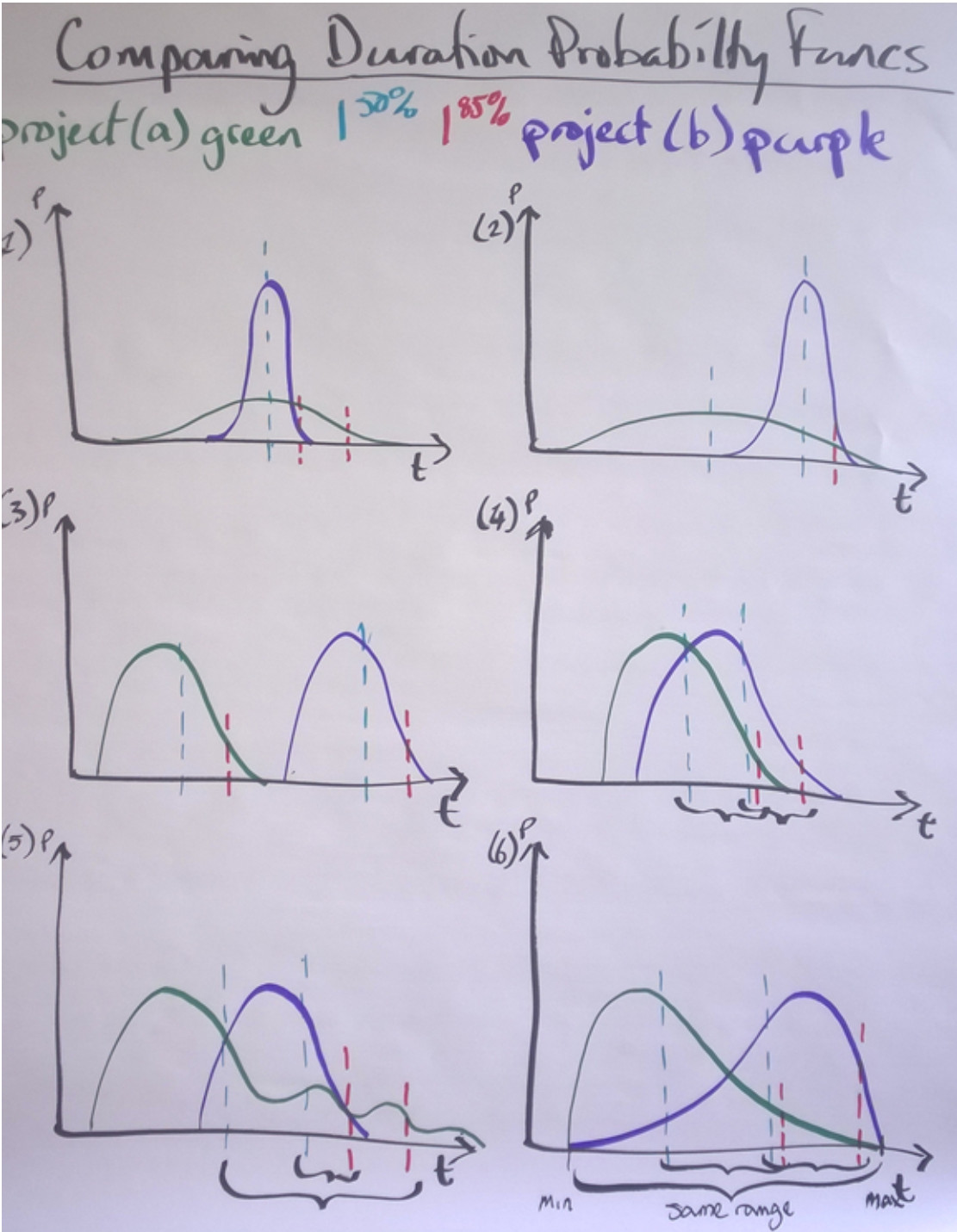
Figure 1. Six scenarios comparing two projects’ simulated durations as probability distribution functions
So, if we were to look at these two projects we see we now have distinct profiles for their distribution. However, if we were to use a WSJF (or CD3) equation to prioritize them and select one over the other as the next to be started in our portfolio, we need a single value for the denominator – the duration value. We cannot use a PDF. The question is which value to choose?
Shortest Possible Duration?
Joshua Arnold, the promoter of CD3, advocates that you pick the minimum value. One of our mutual clients refers to this as the “dream duration”, i.e. the best possible case, the shortest duration possible. Within our PDF this would be the 1%ile number, which would always be visually to the left-hand end of the function.
If we look at scenario 1, project (a) has a much shorter, shortest duration, but actually project (b) has about a 40% chance of definitely completing before project (a). Meanwhile, the variance between the shortest values for (a) and (b) has only a 1 in 10,000 chance of occurring and there is about a 6 in 10 chance that (b) will complete before (a). So dream duration is a bad choice in this scenario at least 6 out of 10 times.
If we move to scenario 2, there is now a greater chance that (a) will complete before (b), probably about 75% of the time, but the variance in the minimum values for (a) and (b) is likely to lead to very skewed results from the equation. If we simply want to choose between these two projects then it is trivial but if there were more choices to be stacked ranked then picking the minimum number is highly problematic.
In scenario 3, using minimum duration is probably okay but we are still assuming “best case” scenario and that generally isn’t a prudent approach to risk management.
In scenario 4, minimum duration is probably a fair method of comparison but we also have to recognize the approximately 30% chance that (b) completes before (a) and hence the minimum value is only safe 70% of the time and we cannot determine this a priori.
In scenario 5, project (a) produces a multi-modal duration PDF. This suggests that the project is subject to external risks that cause delay. Assuming we cannot determine whether these risks will actually occur in advance then the use of the mimimum value for duration of (a) and (b) is flat out dangerous. If we can determine whether one or more risks actually exist then we’d want to use a minimum number for duration given the known risk, i.e. we’d want to simulate the project duration with the possibility of the risk not happening, excluded from our data set. We’d then be left with two single modal PDFs for (a) and (b) that may resemble one of the first 4 scenarios.
In scenario 6, the minimum (and maximum) numbers are identical but project (a) has a far higher probability of completing before (b) – approximately 85% of the time. In this case, choosing the minimum duration for comparison purposes is a useless nonsense.
Median or Mean?
Given that simulated project durations tend to be thin-tailed functions the difference between the median (50%ile) and the mean (the arithmetic average of the data set of possible outcomes) isn’t significant. We could choose to use the median or mean so long as we are consistent. In this case, I have sketched the median values onto the PDFs in figure 1.
- In scenario 1, both projects have the same median value and yet the duration of project (a) is fragile and highly variable, while the duration of project (b) is robust with low variability. The result is that (b) is far more likely to complete before (a). Using the median value, same for both projects, will produce unreliable results.
- In scenario 2, the median value gives a fairer comparison and is definitely a better choice than the minimum value.
- In scenario 3, the median value gives a fair comparison and if we have to use something, this is a very reasonable choice.
- In scenario 4, again the median value gives a fair comparison but it does mask the possibility that (b) completes before (a) perhaps 30% of the time.
- In scenario 5, the median is misleading as (a) looks better than (b). The mean values would actually be closer together and show (b) in a more favorable light. Regardless of which, given the risks associated with the long multi-modal tail in project (a), (b) doesn’t get a fair chance when using median or mean for comparison.
- In scenario 6, the median actually provides a fairly reasonable comparative assessment of the risks associated with completing the projects.
So in general the median or the mean appears better than the minimum for these six scenarios.
What about the 85%?
The red dotted lines on figure 1 show the 85%iles in the project duration PDFs. Now we are dealing in a somewhat worst case, there is a 1 out of 7 chance the projects will take this long and hence a 1 in 49 chance (or about 2%) that they would both take at least this long. This is a much more conservative method of comparison than the best case we examined first.
Now, in scenario 1, (b) looks more attractive than (a) which is a fair assessment.
In scenario 2, (a) and (b) look similar but actually (a) should be far more attractive as it has about a 60% chance of always completing before (b).
In scenario 3, the 85%ile gives us a fair comparison and (a) looks more attractive. Is this a better choice than the median or the mean? Hard to say, but the percentage difference in the two 85%ile values will be lower than if the median or the mean are used for comparison and hence (b) looks relatively more attractive when the 85%ile is used in comparison to the 50%ile or the mean.
In scenario 4, (a) looks more attractive than (b) and that is a fair comparison
In scenario 5, (b) now looks more attractive than (a) and that may also be a fair comparison
In scenario 6, (a) looks more attractive than (b) and again it is probably a fair comparison and the ratio between them probably gives a fair appraisal of the different duration risks.
What about the worst case?
We could examine the longest possible duration value, the 99%ile in the PDF and it would give us similar but opposite results to our best-case comparison.
Conclusions
This small exercise should be enough to demonstrate to you that depending on the projects being compared and their respective duration probability distribution functions, the method used to make a comparison of their durations as a single number – the best case, the worst case, the median value, the mean value, or the 85%ile value, will produce different results, some of which are fair appraisals of the comparative risks and other which are not. No one solution works best in every scenario.
My conclusion from this is that to compare durations of projects you need the whole probability distribution function and you need to make side-by-side visual comparison and then weigh other factors such as the value to be delivered and when. Reducing duration to a single number, regardless of how that number is derived is nonsense. We need to cut it out and start managing the duration risk appropriately. Part 6 of this series will look at a viable method for making properly risk assessed choices for scheduling, sequencing, and selection of projects and other types of work.