What We Know About Duration: Individual Activities
The latest fad in the Agile software development community is to promote the use of Cost of Delay for prioritization. Many readers will know that I have been an advocate of Cost of Delay style prioritization and my 2003 book, Agile Management for Software Engineering contained several Cost of Delay related algorithms. However, I feel there is a lot of misinformed, simplistic and potentially dangerous guidance floating around on Cost of Delay and it is time to provide some clarity.
Most of the Cost of Delay material in the Agile space has focused on referencing and modifying the WSJF (Weighted Shortest Job First) equation from Donald G. Reinertsen’s most recent book, The Principles of Product Development Flow: Second Generation Lean Product Development.
The essence of the WSJF equation is total lifetime profits divided by duration of the product development project.
In the first few posts in this series, I want to look at what we know about the denominator in this equation – the duration of the project. WSJF is also being applied in some frameworks to the prioritization of user stories, features and so forth. I don’t believe this is remotely appropriate and I want to start there by explaining what we know about duration of such user stories or features and illustrating why use of duration on the denominator of the WSJF equation is not appropriate for comparative assessment, sequencing and prioritization of fine-grained work items such as user stories.
What We Know About Duration: Individual Activities
On February 24, 2001, I first published my 5 point power law scale for assessing the size and effort of Features in the Feature-driven Development method, on my uidesign.net blog.
Comparing my data later with some well-known XP advocates such as Tim McKinnon I realized that the London school of User Story writing was producing user stories of similar size and complexity. This scale appeared formally in my 2003 book, Agile Management for Software Engineering. I first used it on a project in Dublin, Ireland in the summer of 1999.
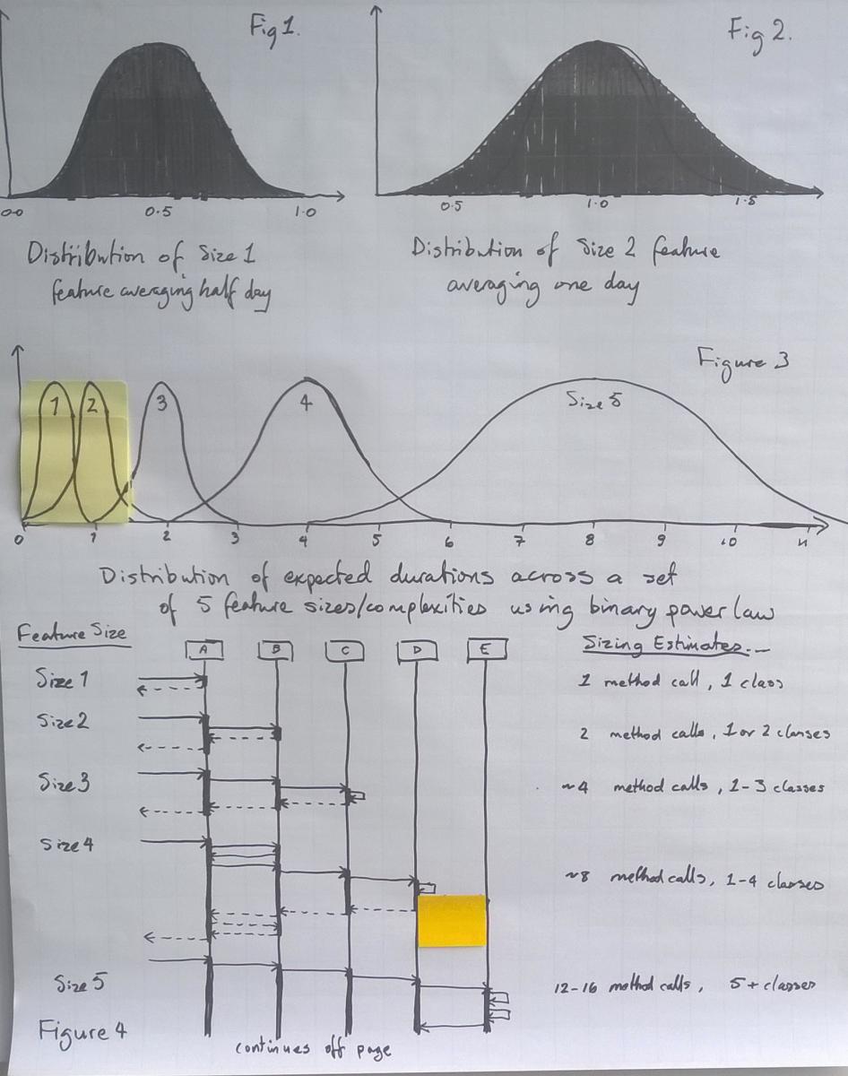
Figure 1 – Idealistic Normal Distribution for Features analyzed into 5 size & complexity categories.
Figure 1 illustrates the scale. It isn’t a random thing. It isn’t based on “estimation” or conversations. It is based on analysis. In other words, it is entirely deterministic. The controlled sentence structure for writing features in FDD enables someone skilled in the art to quickly assess how that feature will impact the code. The sentence contains clues to the method name, the class the method will be coded within and the return value from the method. Given knowledge of the return value, someone skilled in this technique, can almost at a glance make an assessment of how many classes will need to be navigated to produce the desired output. The assessor isn’t doing a design just using their judgment to assess what the design is likely to entail, in terms of classes accessed and method calls.
So I created a 5 point scale: features of sizes 1 through five. I assessed that the average level of effort for such features would rise in a power 2 function: 0.5 days; 1 day; 2 days; 4 days; 8 days or more.
Assuming we’ve made a correct sizing – which is a reasonable assumption as more than 90% of features are likely to be correctly sized using this technique, it is still unlikely that a task duration such as design and coding the feature – actually writing all the method calls and all the unit tests – will take precisely the average time. In fact, it is likely to be random and reasonably evenly spread.
If we had enough data points – a few hundred – and we have a situation where there is no multi-tasking, no delay or blocking on other dependencies and no disruption during the task, then we might expect a properly normal distribution with a scale of about 50% above and below the average. So Size 2 features taking on average 1 day should take something between 0.5 and 1.5 days to complete.
There is a degenerate case where multi-tasking does not skew the shape of the of the normal distribution. This is where the rate of task switching is twice or more as fast as the shortest possible task duration, i.e. if we have a 31 minute task and we switch tasks every 15 minutes then there is an equally random chance that all tasks will be interrupted and hence the distribution will remain Normal. Of course, such rapid task switching would mean the process was massively inefficient and the whole distribution would be right shifted and scaled to the right as a consequence. This is why it is a generate case: it exists in mathematical theory but in reality it never exists.
If we consider now that the smallest task might take 30 minutes (0.5 hours) and the longest might take 12 days (96 hours) we have a spread of variation for Feature effort that spans 200x the smallest duration. The 200 multiple is right in line with reports from Reinertsen. It is probably reasonable to assume that task completion times will span at least 50 times the minimum size regardless of the process used. Again this data is “level of effort” and is still assuming no task switching, no delays and disruptions in service.
Now let us consider the spread of variation of Feature sizes in a given project…
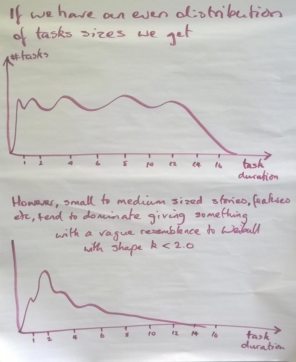
Figure 2 – Even distribution of features and a more typical mix weighted to small and medium sized Features
Figure 2 shows how the distribution of task duration might vary as we sum the distributions for each feature size. In other words, if we treated all features, simply as features, how long might they take to complete? The upper diagram shows a multi-model distribution for an evenly spread distribution of features, i.e. we have approximately the same number of size 1s, as we do, size 2, size 3, size 4, size 5. I have never seen such an even spread. More typical is a skew towards small and medium size with size 2 being the most common. This produces a distribution more like the lower example.
What do multi-tasking, delay and disruption do to the distribution shape?
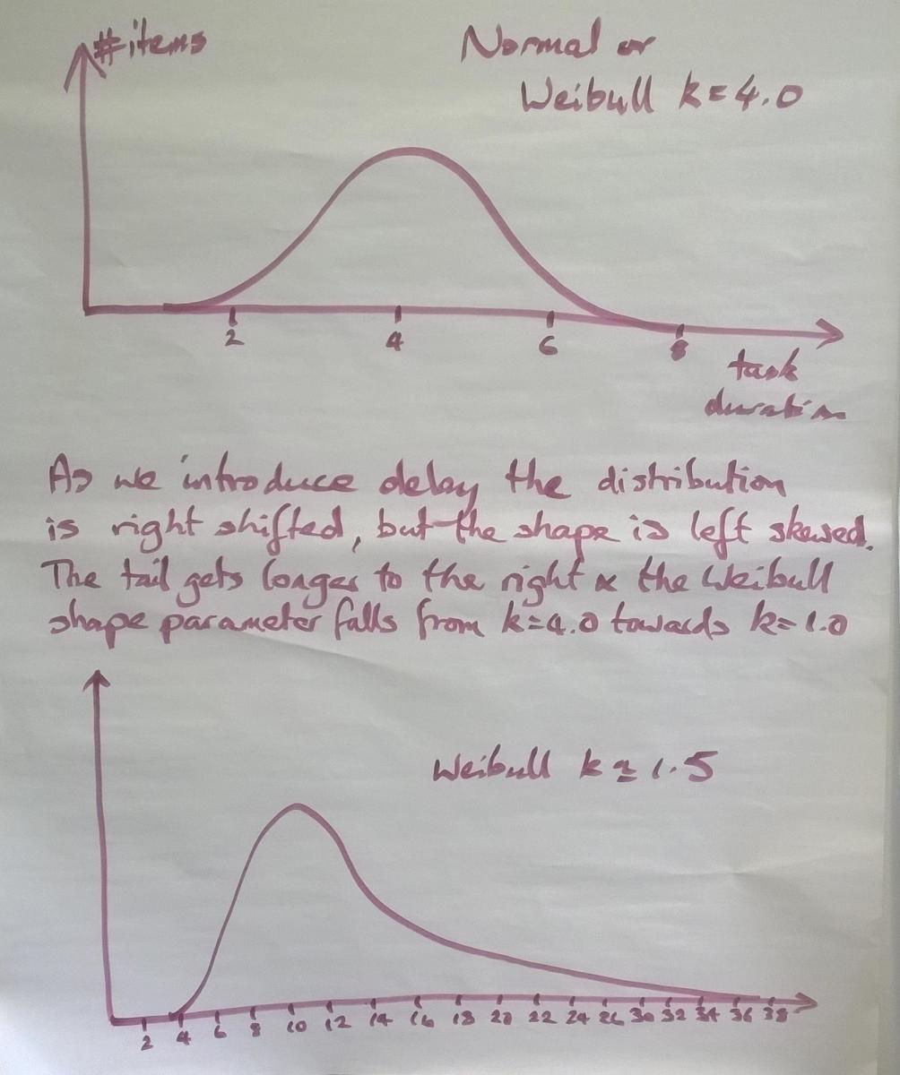
Figure 3 – Multi-tasking, delay, and disruption right shape and left shape the distribution
If there is less than an even chance of something being delayed then the tail of the distribution gradually gets pulled to the right. Therefore, long-duration tasks have more chance of being delayed and things which are delayed have more chance of being delayed further. This is what produces the long tail to the right.
Mathematically, as we pull the tail to the right, the shape parameter in the Weibull equation shrinks. We refer to this as left-shaping or left-skewing the distribution. The whole distribution has been physically shifted to the right. Note carefully that I have placed a scale on the x-axis. The mode|median|mean in the Normal distribution is at 4.0 while the lower curve has a mode of 11, a medium of approximately 11, and a mean of approximately 12. So the mean task duration has increased 3 fold because of delay and multi-tasking.
Averages are easily explained but it is the tail on the distribution which represents much of the risk. In the normally distributed ideal situation, the task is being completed in a maximum of 8 while after we introduce multi-tasking, delay and disruption of service the maximum has grown to 38.
Figure 3 showed the skew in the distribution for a size 4 feature where some multi-tasking and delay due to dependency and disruption of service (i.e. unavailability of the worker through for example illness or jury duty) occurs. You can imagine when we model this for all five sizes and then roll it into a single distribution similar to figure two that we get an even more pronounced long-tail effect.
All of this is for a single activity. We haven’t even started to look at a workflow of multiple activities with delays waiting between activities in the workflow. I will cover that in the second post in this series.
So What Do We Know About Task Durations?
In summary then, if and only if you have a deterministic analysis technique to quickly and cheaply asses size and complexity you may be able to break your task durations into a taxonomy of categories.
As Jurgen Appelo pointed out in his book Management 3.0, Fibonacci series so beloved of Agilists does not in fact appear in nature. Also it’s index isn’t sufficiently sparse: a story assessed as a 3 on a Fibonacci scale is likely to be a 1, 2, 4, or 5, while the alternatives above and below on the Fibonacci scale are 2 and 5. Hence, it is quite random whether a user story is a 2, 3, or 5. There is probably less than 50% chance it is actually a 3. If we assume that there is never any pre-emption while the task is undertaken, there is still a very low correlation between its size or complexity and its actual duration. Of course, pre-emption does happen and hence there is really no correlation between its story point sizing and its duration. This makes it useless as a means of comparative assessment and prioritization in an equation such as WSJF as there is a high probability that the denominator in the equation for each task or item is wrong. This can have a strong effect on the outcome or a ranking based on the results of the equation. As a consequence of this there is little to no information value in the sizing and for the purposes of calculating duration, we may as well assume all user stories are the same size. We are unable to deterministically assess the duration of any one item of a given type against the duration of another item of the same type. This analysis eliminates user story size as a usable parameter in the WSJF equation.
On the other hand, power laws and Weibull distributions including (k=4.0) Normal distribution and (k=1.0) Exponential distribution do exist in nature. So it is much more likely that sizing for user stories follows a power law. Jurgen discovered in 2009 that I had published such a power law, and the earliest online reference is February 24th, 2001. Even with a power-law scale there is some, but less chance of the actual duration overlapping with an item of a different size or complexity. Hopefully, figure 1 was sufficient to persuade you that a point sizing scale assessing size and complexity is not meaningful in assessing task duration for the purposes of comparative assessment and prioritization? If not perhaps the second article in this series will get you to the conclusion that estimating duration for the purpose of using it as the denominator in the WSJF equation is not useful at the granularity of tasks, stories, features or epics.
We know from other reports that task durations typically have a spread of up to 200x and the FDD power law scale I developed demonstrates that quite readily – if we assume an 8 hour working day. In my 2003 book, I assumed only 5.5 productive hours in the day. Using this smaller number still produces a multiple of 132 from smallest to largest feature.
So we understand that the problem of estimating task durations such as user story development is non-linear, but we also understand that it is non-deterministic. If we know for example, for certain, from deterministic analysis, that this feature involves 3 classes and 5 method calls, we still cannot say with deterministic precision how long it will take. The duration is a Weibull distributed random variable.
So, in summary, for an individual activity in a workflow, the task duration to complete the activity, varies non-linearly, is non-deterministic, is approximately Weibull distributed with a shape in the range 1.0 < k < 4.0 and most likely in the range 1.3 < k < 2.0 and can have a spread from shortest to longest that can be up to 200 times the shortest value.
If you are trying to “estimate” the duration of a task such as designing, coding, testing a user story, you are basically guessing. You are rolling the dice, making a stab in the dark. The actual elapsed calendar time (or duration) for the activity is likely to be wildly different from your “estimate.”
In the next post in this series I will look at what happens when we have a chain of activities put together as a workflow. What do we know about lead time through a workflow?