What We Know About Duration: Workflows
This is the second in my series of posts about Cost of Delay. This post looks at what we know and understand about duration (lead time). To catch up, you can read the first in the series, What We Know About Duration: Individual Activities.
Aside: Recently I attended the Real World Risk 5-day class with Nassim Taleb. Referring to science generally and risk management specifically, Taleb said, “there is no ‘let’s assume'”. I intend to include this statement on all blog posts related to risk management, forecasting, planning and so forth. Every time you see me having to use the phrase, “let’s assume” in order to defend or advocate for an existing method I believe to be flawed, we are already venturing into the realm of fantasy. “There is no ‘let’s assume’.”
The use of Cost of Delay to prioritize or sequence work is becoming increasingly popular in the Agile community. There are several authors promoting somewhat similar quantitative, mathematical approaches to ranking requests in order to prioritize or sequence a series of competing request. Donald Reinertsen has promoted the use of the Queuing Theory technique known as Weighted Shortest Job First (WSJF) and Joshua Arnold is promoting what he believes is a simpler derivative known as CD3 (Cost of Delay Divided By Duration). Some other authors are promoting derivatives of these two ideas and often, and confusingly, calling them by the same name, even though they have changed the parameters in the equations. Both WSJF and CD3 use “duration” as the denominator and hence, I’ve been examining what we know about duration for different aspects of knowledge work requests. Part 1 looked at single activities and now Part 2 looks at a customer request that passes through a series of information or knowledge adding activities in a service delivery workflow.
The Kanban community has been measuring, reporting, studying and acting upon, duration information since its inception in 2007. We had individual activity and workflow duration data on the first kanban system at Microsoft in 2004. In the Kanban community, duration is usually referred to as lead time. This is unambiguously defined as the time from a commitment to the customer to accept, work on and deliver their request until it is actually delivered or accepted by that customer. With a decade or so of experience and data, we’ve learned a lot about duration.
Figure 1 shows a typical Kanban board and system. This one features several buffers and wait states. The important thing to recognize is that the buffers or wait states are not queues and typically don’t have a defined queuing discipline. More accurately these buffers and wait states behave more like what industrial engineers refer to as “supermarkets”, I find it more useful to think of them as “beauty contests.” An item will be selected from a wait state or buffer if there are available workers with the correct skills and if the item’s risk profile is such that it is the best choice given the set of available options. At times, it may be the only option. At other times, it may be the only option but it still waits because the idle workers are not suitably skilled. The key lesson is to recognize that the waiting time, or delay, in a buffer or wait state, cannot be determined in advance, and is entirely arbirtary and hence, non-deterministic in nature.
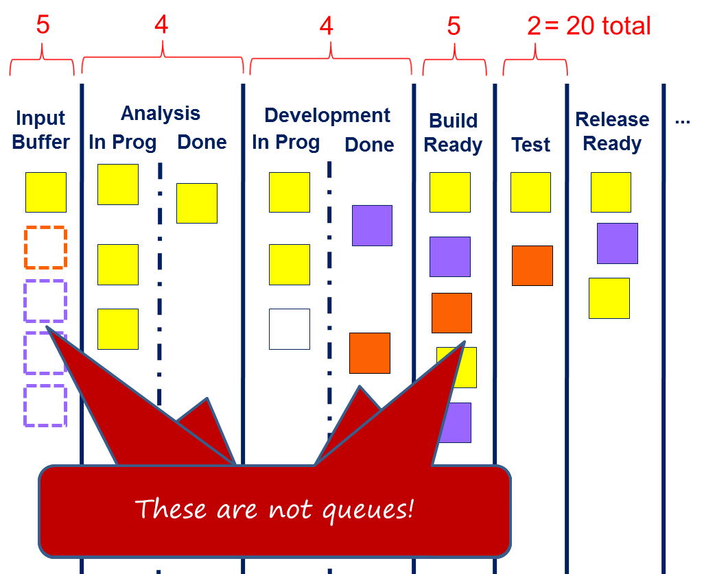
Figure 1. Typical Kanban Board showing buffers & wait states without queuing discipline
The next thing to understand is just how much delay is actually typical in a professional services, knowledge work, workflow. The ratio of total duration to time spent waiting is known as the Flow Efficiency. Figure 2 illustrates how flow efficiency is calculated. In the very best case studies reported in the Kanban community, flow efficiency reaches upwards of 40%. On the very first Kanban in 2004 it started at 8%. It turns out that 8% is a high starting figure and there have been reports of 1%-2%. Typically, we expect flow efficiency to be in the range 1%-25% with the majority of cases being towards the bottom end of that range. Hence, the corollary is important – for work item duration between 75% and 99% of time is waiting time, and the waiting is entirely non-deterministic in nature.
The other 1% to 25% is covered by the first article in this series, What We Know About Duration: Individual Activities. The conclusion of this early article is that an individual task duration can vary by a factor of up to 200 times from minimum to maximum and is non-deterministic in nature. We now know that this non-deterministic task duration time contributes between one one hundredth to one quarter of the total duration. So we have delay time which is entirely non-deterministic contributing 75-99% of the total duration and the sum of task durations which can vary in scale by 2 orders of magnitude and these contribute the remainder. Let’s assume that we believe we can size items and that their size and complexity does correlate to individual task duration, then we still have a problem with the non-determinism of the buffers and wait states which dominate the actual workflow duration. Even if we could accurately say, “this user story will take 4 days”, it is likely that the total duration is 16 to 400 days. Imagine we were comparing it against another item which we believed would take only 2 days. Our deterministic analysis would suggest without doubt that the 2nd item will complete before the 1st. However, the reality of the non-deteminism in the buffer and wait states means that there is close to a 50% chance that the the 2nd item which we assessed as taking half the time of the 1st item, will in fact take longer. In addition to there being close to a 50% chance that it will take longer, there is a possibility that it may take up to 100 times longer.
In risk management, the 50% likelihood it will take longer is know as “the likelihood of x” while the actually amount longer is known as “the function of x, or f(x).” In risk management we need to worry more about f(x) – or the impact – than we do about the likelihood. If we were using our 4 days versus 2 days values in a prioritization equation to make sequencing decisions, there is an almost 50% chance we make the wrong decision in terms of sequencing one over the other, and the impact of the wrong decision may be significant. Given that the two items don’t exist in a vacuum alone, the complexity of the problem rises dramatically when we consider the considerable number of other alternatives we will be comparing them against. It only takes a few more items in the comparison before we reach a point that the likelihood of correctly sequencing them based on duration quickly approaches zero. And of course, all of this analysis involved the “let’s assume” that we can actually determine the individual task duration correctly, which we know to be false, from part 1 of this series of articles.
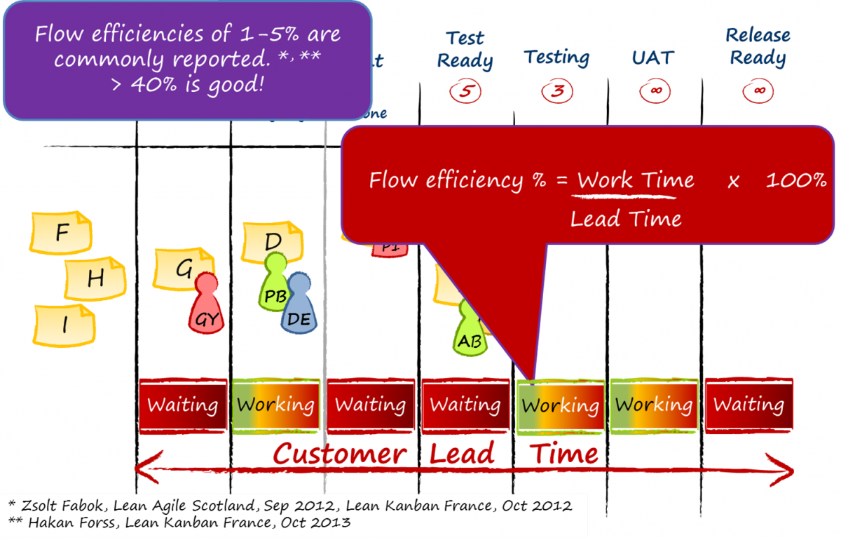
Figure 2. Illustrating Flow Efficiency in a Kanban Workflow
Figures 3, 4, and 5 were supplied by Ramesh Patil, the CTO of Digite, and are extracted from real software development data tracking feature development in the SwiftKanban product.
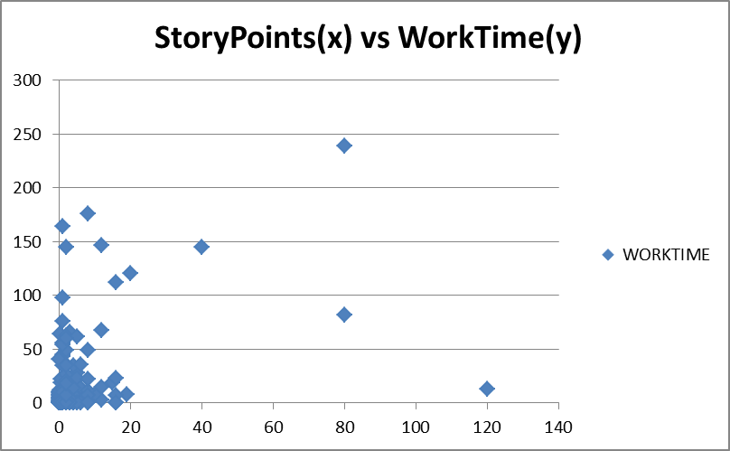
Figure 3. Story Points versus Work Time
Figure 3 shows epic story point sizing versus actual recorded work time for activities such as development. If there was a correlation between the size of an epic, made up of an aggregated set of individually sized user stories, then we would expect to see the points cluster in a roughly linear diagonal line from the origin towards the upper right corner of the graph. We don’t see that and in fact the scatter of the points suggests there is no correlation.
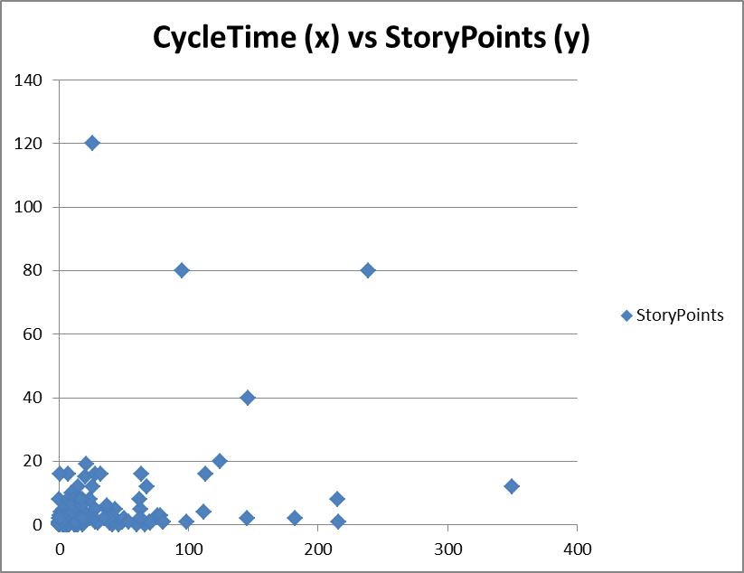
Figure 4. Lead Time versus Story Points
In Figure 4, the term “cycle time” actually reports the Lead Time, or duration from commitment to ready for delivery. In this example, we are plotting story points for epics aggregated from a set of individually sized stories, against the actual duration taken to complete. If there was a correlation then we would expect to see a clustering of the points in a roughly linear line from the origin point to the upper right hand corner of the graph. We do not see this and as a consequence we can conclude that story point sizing does not correlate to duration and cannot be used for Cost of Delay calculations using WSJF or CD3 equations.
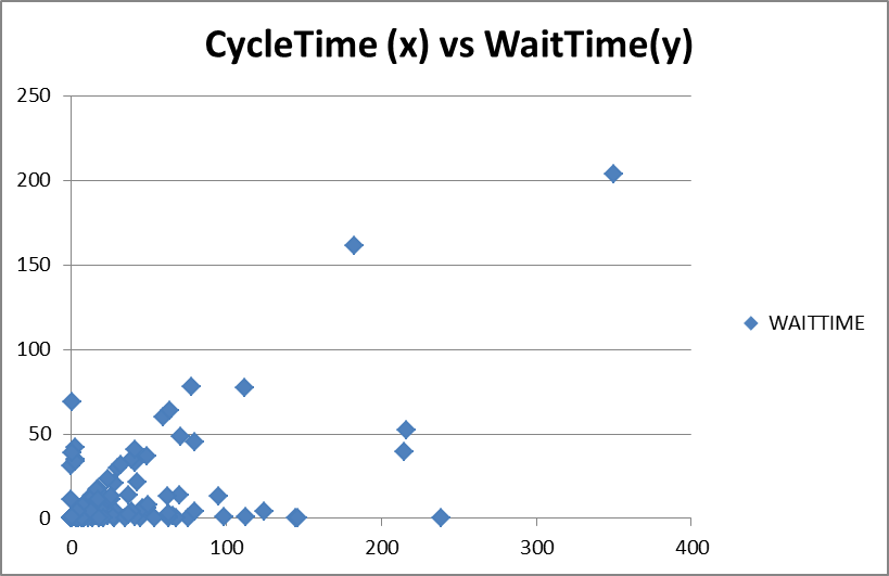
Figure 5. Lead Time versus Wait Time
Figure 5 shows a plot of total duration or lead time versus the time a ticket spend waiting. In this plot we see some emergence of a correlation. There is a strongly defined linear plot of points rising diagonally from the origin towards the upper right. We also see some points along the x-axis. These are points with a high level of flow efficiency. This is typical of “expedite” class of service items. Items in between, in the lower right half of the graph below the linear diagonal suggest items of higher flow efficiency, perhaps receiving a higher class of service, these might be items with some sort of fixed delivery date, but given the nature of the product development, they are more likely defects given a higher class of service in order to avoid blocking mainstream development.
The upper left of the diagram is almost devoid of points because we would not expect to see any points where the total duration was lower than the waiting time. The few points clustering around the y-axis may be noise in the data set, or require some further investigation.
Classes of Service
Figure 5 demonstrates that the strongest way to influence duration is, in fact, to use a class of service. By giving an item a higher class of service, we effectively make it more “beautiful” than other tickets. It receives preference for pull decisions. As a consequence it spends a lot less time waiting and its lead time falls dramatically. For a truly expedited ticket we would expect its duration to look like that of an individual task from as illustrated in the first part of this series of articles, or the sum of several individual task durations.
Lead time (or duration) is Weibull distributed
Figure 6 shows a summary of distribution curves for lead times. These follow a Weibull distribution with different shape parameters.
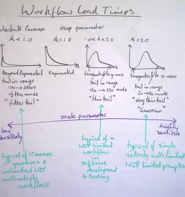
Figure 6. Workflow Lead Time Weibull Curve Shapes
As described in part 1 of this series, individual activities when not pre-empted will exhibit a near Gaussian shape with a Weibull curve with shape parameter kappa, k, lying in the range 2.0 < k < 4.0. However, given that pre-emption does happen and some delay is incurred and also given that a specific item of a defined type may still have size and complexity that varies by two orders of magnitude, it is likely that we will see task durations with a distribution curve that has a shape parameter in the range 1.5 < k < 2.0. Some data sets we have such as the development activity data from the first Kanban at Microsoft in 2004 show a shape parameter just greater than k=2.0 but for the test activity the shape is closer to k=1.7. This suggests that testers were pre-empted or delayed more often than developers.
For workflows where we are using Kanban, limiting work-in-progress, limiting pre-emption in activities, limiting the available choices in wait states and buffers and hence, improving the flow efficiency into the 25%-40% range, we typically see lead time distribution curves with shape parameter 1.0 < k < 2.0 and usually in the range 1.3 < k < 1.6.
As we move to pre-Kanban, unlimited WIP, and a lack of focus on removing delay, a lack of avoiding or mitigating blocking issues then we slowly see the shape parameter decay towards and then below k=1.0 (the exponential function). We refer to this as “left shaping” or “right skewing” the distribution as the tail extends longer and longer towards the right hand side. A longer tail means that we have less and less predictability and more and more impact from delay. Perhaps there is a only a small percentage of items being delayed for longer periods, a low probability of x, but the length of the delay, the impact, of f(x) is considerable. This is where trouble occurs, particularly in lower maturity organizations that panic under stress. Shape parameter values of k below 1.0 represent high-risk situations and a high likelihood of undesirable outcomes. We associated long fatter tailed distributions with k<1.0 with IT operations, IT services and very low maturity software development. Data sets in the range of k~0.75 have been published.
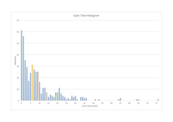
Figure 6. IT Services Lead Time Data (courtesy Andreas Bartel)
Andreas Bartel from Hamburg posted this IT Services lead time (duration) data to Twitter at the beginning of March. The Mode in the data is less than 1 day, the median is 6 days, the mean is 9 days and the tail in the data set is 77 days, or about 100 times greater than the mode. This data set has a Weibull shape parameter k~0.8.
Modeling Lead Time Data Sets
There are two schools of thought emerging in the community. One school led by such luminaries as Troy Magennis, Larry Maccerone, and Ramesh Patil believe there is little point in trying to make “best fit” distribution curves and instead they prefer a style of statistical modeling and simulation known as “bootstrapping” where they only use data points in from a historical data set and ignore the gaps. The other school of thought believes that true Monte Carlo simulation requires parametric models. Essentially the argument is one of model error versus forecasting error. Given that either approach produces forecasts that far exceed other existing methods in the Agile field, it is somewhat of an esoteric point and very much at the “bleeding edge of Kanbanland” in terms of experimentation and resolution.
Figure 8 shows a lead time distribution for software development and testing of telecom node middle layer architecture functionality. This was captured at one of my clients, extracted from the Jira tracking software, during the summer of 2014.
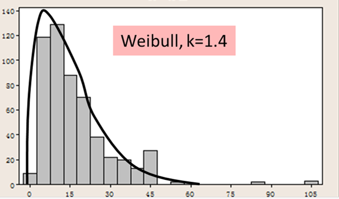
Figure 8. Lead time for telecom grade software development & testing
The data set fits reasonably well to Weibull with shape parameter of k~1.4 and scale parameter of 61. However, there are some outlying data points. The tail is longer and fatter than the Weibull curve would model. This is typical of many real-world data sets
Figure 9 shows a model similar to the real data in Figure 8. It can be modeled using two Weibull curves, one thin-tailed with shape k>1.0 and the other fatter tailed with shape k<1.0. With just two curves in aggregate, we achieve a parametric model that fairly closely models the real data set. This aggregate parametric model, or distribution curve, could be used in a Monte Carlo simulation to forecast the outcome for a larger set of items flowing through the same service workflow, or for setting service level expectations or agreements for service delivery.
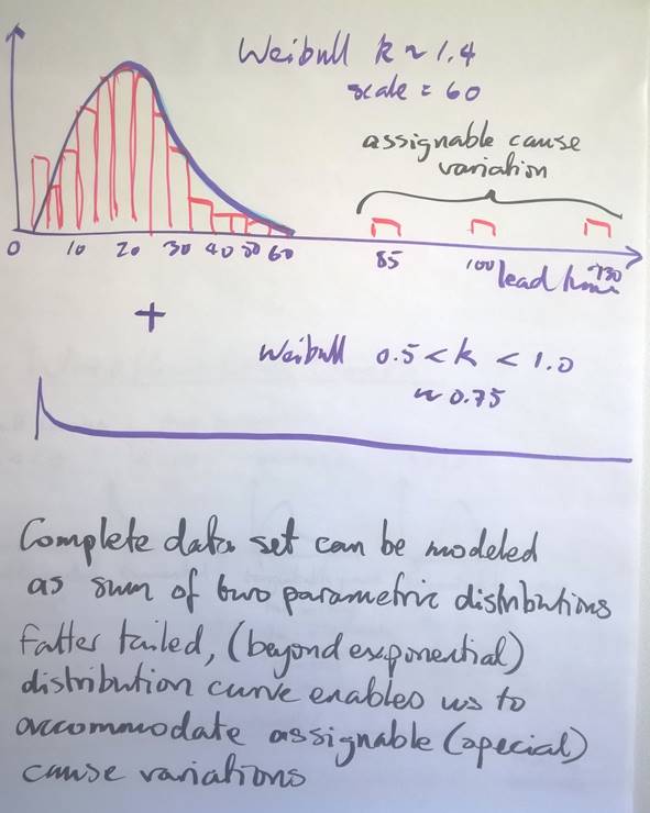
Figure 9. Composite Parametric Model using 2 Weibull Curves to model a real lead time data set
Conclusions
What we know about duration:
1. Durations (or lead times) follow Weibull distribution curves but with longer, fatter tails. Typically, two curves in the composite are required to adequately model a real data set
2. It is typical for a lead time distribution curve to exhibit a spread of variation between the mode and the tail that is 4x – 200x. The spread of variation from the lowest to the highest value may be in the range 50x – 200x.
3. Lead times are entirely non-deterministic
4. The biggest influence on lead time is achieved by reducing waiting times.
5. The best way to positively affect (reduce) lead time is through the use of classes of service which reduce time spent in wait states and buffers.
6. Limiting Work-in-progress (WIP) using a kanban system has a dramatic positive effect (reduction) on lead time as it reduces choice in wait states and buffers and increases the likelihood that an item will be chosen for the next activity
7. Weibull curve shape parameters for lead times through service delivery workflows vary in the range 0.5 < k < 2.5 in observed real world data sets
8. Variation in size or complexity for items of the same type does not correlate to lead time (duration)
9. Class of service for items of the same type does correlate to lead time as flow efficiency is greatly improved
10. Expedite class of service items for items of the same type will exhibit lead time distributions with a Weibull shape parameter k in a range around 2.0
11. Flow efficiency is seldom obvserved above 40%. Typically flow efficiencies without the use of a kanban system and a process improvement focus on reducing delay and mitigating blocking issues are usually less than 10% and as low as 1%. As a consequence, the size or complexity of an item has very little influence on its duration.
12. Wait states and buffers in professional services, knowledge work workflows are not queues and rarely have any queuing discipline unless explicitly stated in a class of service definition. As a consequence waiting time is entirely non-deterministic
13. As flow efficiency is low and waiting time is entirely non-deterministic, for items of a given type, it is impossible to determine their duration any more accurately than the bounds of the lead time distribution curve.
As a general conclusion, if we are dealing with items of the same type, for example, user stories compared to other user stories, with the explicit intent of using duration to aid in the sequencing of work using a Cost of Delay equation such as WSJF, we are unable to determine or differentiate the duration of any one user story from another in advance. The same is true for work items at different scales such as epics, an aggregate collection of related user stories. We are unable to determine the duration of one epic versus another.
At the scale of a project – at least 2 orders of magnitude larger than a single user story – we can simulate the duration of the project, given a known defined, determined scope of user stories, using Monte Carlo simulation. This will be the topic of a subsequent post in this series on Cost of Delay.