Leveraging Probabilistic Forecasting for Better Outcomes
Kanban originally shocked the Agile community in 2008 as it became known for not using several practices agilists hold dear: no time-boxed iterations; no prioritization; and perhaps most shocking of all, no estimation!!! So how do you plan a project with a method that doesn’t use estimates? The answer is that you use historical data or a model of expected capability to build a probabilistic forecast of the project outcome.
Statistical Enablers For Project Forecasting
Two key ideas enable forecasting projects in Kanban: the first is the lead time distribution for work pulled through the kanban system, and the second is the Little’s Law equation from queuing theory.

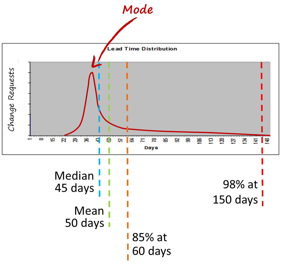
Figure 1 shows a lead time distribution for work items (typically, project features or requirements) flowing through the kanban system. To use a historical lead time distribution like this we need to understand a few assumptions and be sure we’ve chosen our data correctly. We must also believe that our future observed capability will be similar to past performance. This is particularly true in environments with low flow efficiency where the individual’s skill and capability, the technical practices used, and the size or complexity of the requirements have a significant influence on the lead time. Hence, in low flow efficiency environments, we can change the people, dramatically change the method of capturing the requirements, and change the technical working practices while observed lead time distribution is not significantly affected. In higher flow efficiency environments we’d want to pay attention to keeping the skills and experience of the individuals fairly similar to those involved when we captured our historical data and to keep the working practices and the methods of analysis and requirements development fairly similar. This should ensure that we can expect lead time distributions in the future that are sufficiently similar to our existing data that we can reliably use the historical data for a forecast.
Secondly, we need single-modal data for a good forecast. To get single modal data for our lead time distribution, we need separate distribution curves for work of different types or classes of risk. Hence, risk assessment of the requirements and clustering and filtering of historical data by risk categories is key to producing a good forecast.
Thirdly, we need to know how far back historically we should sample our lead time histogram to create our best-fit distribution curve. This is where a lead time run chart comes in handy. We can observe changes to the system design in the run chart data in terms of the mean value and the spread of variation of the data points. If there are discontinuities, usually associated with system design changes (hopefully, improvements) then we only wish to sample as far back as the point where the mean and spread of variation changed. In other words, we want a histogram of data that reflects current conditions and capability unpolluted with older data points. Another way to find this point in time is to monitor the kanban system liquidity and look for dates where the liquidity level changed significantly. Such a date would provide the historical backstop point for sampling data for our histogram.
Once, we have a histogram for each cluster of risks (classes of service) or each type of work within the project scope, assuming our project scope and requirements are tagged by type or risk category, as discussed in part 2 of this series, then we can forecast our project schedule using Little’s Law.

The Kanban variant of Little’s Law states that the mean delivery rate of work items leaving the kanban system, is equal to the number of kanban in the system (the WIP limit) divided by the mean lead time through the system. Hence, if we know the WIP limit of our kanban system, and we know the mean of our lead time distribution, we can calculate how quickly our completed work will arrive ready for delivery at the end of the project.
Building A Schedule Forecast
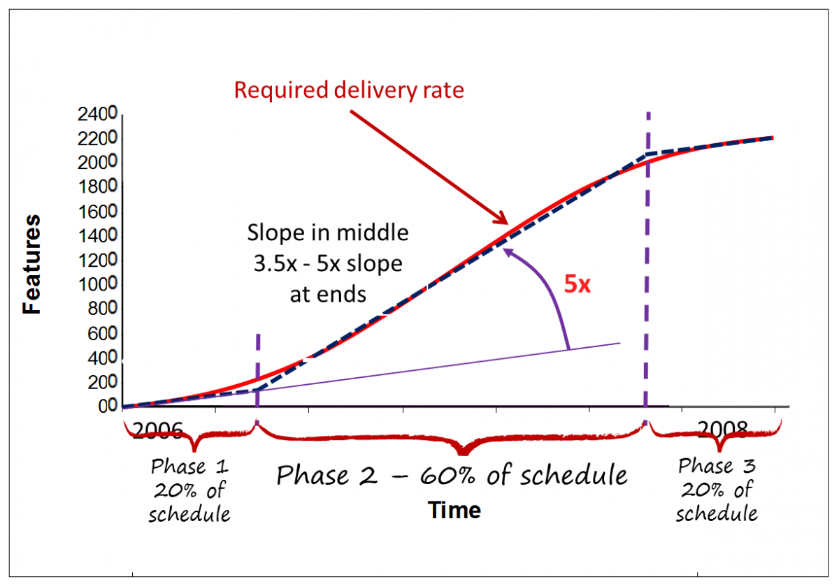
Figure 3 shows a simple three-phase model that we often use for projects of medium to large scale. This model is effective for projects from 6 weeks long to multiple years in duration. The parameters in the model are my own choices and you might like to vary your parameters but 3 phases is probably sufficient. I assume 20% of the timeline for phase 1 – a period of relatively low flow efficiency. The next 60% of the timeline is phase 2 – a period of high flow efficiency, some Agilists refer to this as “hyper-productivity”. We end with a period of lower flow efficiency for the remaining 20% of the timeline. I first documented this model in my 2003 book, Agile Management for Software Engineering. The probabilistic forecasting technique described here predates Kanban. However, the use of kanban systems makes the forecast so much more accurate by improving the consistency of the lead time.

Figure 3 assumes a project with homogeneous requirements – in other words, requirements that are all of the same type and of the same class of risk. What do I mean by this? If for example our requirements are all captured in the same way, for example, User Stories, we might treat them as all of the same type. If some have a vendor dependency while others don’t we would typically see multi-modal data in our lead time distribution because the vendor dependency causes a delay and longer lead times result. It would be wrong in such a case to treat all the requirements homogeneously and hence we would want to filter for the risk of vendor dependency or not. So we’d want our requirements tagged to show whether they were vendor-dependent or not. So we would no longer have homogenous requirements, we’d have two different classes and we’d need to simulate each separately.
Using Capacity Allocation To Manage Requirements RIsks
We would build a simulation for each batch of requirements by class or type. For example, if we have regulatory requirements as described in part 2 of this series then we would want to forecast those separately from the non-regulatory work within the project scope. As discussed in Part 2, regulatory requirements typically have fixed delivery dates and the project delivery date is generally tied to the regulatory compliance date. Hence, we have a batch of regulatory requirements to be delivered before the end of the project. This allows us to introduce a capacity allocation in our kanban system to pull regulatory requirements at a steady pace throughout the project’s lifetime. We know the size of the batch of regulatory requirements. We know the delivery date. We know today’s date. So we can calculate the required mean delivery rate. We know the lead time distribution for pulling regulatory requirements through our kanban system. From these parameters, we can calculate a WIP limit for regulatory requirements. This will become our capacity allocation within the whole kanban system. We might design a lane or use a color of the ticket to signify regulatory requirements on our visual board. We would set a WIP limit for tickets of that color or in that lane. Effectively, we have created a Kanban sub-system designed to pull the regulatory requirements at the pace needed, starting now and ensuring delivery of all of them before the deadline for the project.
Should we sequence our regulatory requirements? As discussed in Part 2, it depends on whether or not some of our regulatory requirements are still subject to change – due to lobbying, the fickleness of the regulator, or a change in political leadership. If not, then our regulatory requirements are homogeneous from a business risk perspective and we can pull them in any order we like. There is no need to sequence them. If some of them are still subject to change then those should be deferred until later in the project. At the beginning and through the early phases of the project we should sequence and select requirements that we know are stable while deferring unstable requirements until any ambiguity is resolved.
Conclusions
While using historical data to form lead time histograms, developing best-fit distribution curves, forecasting completion rates, establishing WIP limits, setting capacity allocations, and influencing capacity allocation policies all sound very complex and involve some basic understanding of statistics, making project plans this way is very fast and easy. Given that the requirements have been assessed and tagged with risk categories, it ought to be possible to build a project forecast within a few hours. Even for significant projects spanning more than 1 year and costing more than $10,000,000, it ought to be possible to build a reliable, high-quality forecast in less than 1 day using only a couple of people to gather and analyze the necessary data.
A probabilistic forecast made in this way is likely to be significantly more accurate – more similar to the actual outcome – and is also significantly faster and cheaper to create, than a traditional deterministic plan that requests an estimate for each work item within the project scope. The major advantage of probabilistic forecasting is that we do not need to interrupt workers doing customer-valued work to ask them to estimate future, and often speculative, work. Eliminating this wasteful disruption has been shown in many Kanban case studies to significantly improve delivery rates, lead times, predictability, and quality.
While this article described the 3-phase, so-called Z-curve, forecasting model, those using LeanKit or Swift Kanban products can utilize the Monte Carlo simulation feature to produce even more robust forecasts for project outcomes. Forecasting is fast, cheap, and more accurate than traditional estimation and planning methods. Kanban systems enable forecasts to be used actively to manage project risks and ensure good project governance by making explicit scheduling and capacity allocation policies.
Learn More with Enterprise Services Planning
If you’re intrigued by how Kanban leverages historical data and statistical models to revolutionize project planning, it’s time to dive deeper. The Enterprise Services Planning (ESP) course is designed to equip you with the tools and knowledge to implement these advanced techniques in your organization. Learn how to create reliable forecasts, optimize service delivery, and manage complex projects with confidence. Take the next step toward mastering modern project management—enroll in the ESP course today and transform the way you plan and deliver results.


